21. Case study: sync#
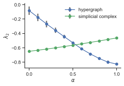
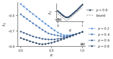
Here, using XGI, we reproduce figures 1 and 2 of the paper
“Higher-order interactions shape collective dynamics differently in hypergraphs and simplicial complexes”
Yuanzhao Zhang *, Maxime Lucas *, Federico Battiston
Nature Communications 14.1 (2023): 1605
https://doi.org/10.1038/s41467-023-37190-9
import matplotlib.pyplot as plt
import numpy as np
import seaborn as sb
from mpl_toolkits.axes_grid1.inset_locator import inset_axes

import xgi

sb.set_context("paper")
sb.set_theme(style="ticks")
# utility functions to compute the Lyapunov exponents from the Laplacians
def compute_eigenvalues(H, order, weight, rescale_per_node=True):
    """Returns the Lyapunov exponents of corresponding to the Laplacian of order d.

    Parameters
    ----------
    HG : xgi.HyperGraph
        Hypergraph
    order : int
        Order to consider.
    weight: float
        Weight, i.e coupling strenght gamma in [1]_.
    rescale_per_node: bool, (default=True)
        Whether to rescale each Laplacian of order d by d (per node).

    Returns
    -------
    lyap : array
        Array of dim (N,) with unsorted Lyapunov exponents
    """

    # compute Laplacian
    L = xgi.laplacian(H, order, rescale_per_node=rescale_per_node)
    K = xgi.degree_matrix(H, order)

    # compute eigenvalues
    eivals, _ = np.linalg.eig(L)
    lyap = -(weight / np.mean(K)) * eivals
    return lyap


def compute_eigenvalues_multi(H, orders, weights, rescale_per_node=True):
    """Returns the Lyapunov exponents of corresponding to the muliotder Laplacian.

    Parameters
    ----------
    HG : xgi.HyperGraph
        Hypergraph
    orders : list of int
        Orders of interactions to consider.
    weights: list of float
        Weight of each order, i.e coupling strenghts gamma_i in [1]_.
    rescale_per_node: bool, (default=True)
        Whether to rescale each Laplacian of order d by d (per node).

    Returns
    -------
    lyap : array
        Array of dim (N,) with unsorted Lyapunov exponents
    """

    # compute multiorder Laplacian
    L_multi = xgi.multiorder_laplacian(
        H, orders, weights, rescale_per_node=rescale_per_node
    )

    # compute eigenvalues
    eivals_multi, _ = np.linalg.eig(L_multi)
    lyap_multi = -eivals_multi
    return lyap_multi
21.1. Fig. 1#
21.1.1. Generate random structures#
N = 50  # number of nodes
ps = [
    0.1,
    0.1,
]  # ps[i] is the wiring probability of any i+2 nodes (ps[0] is for edges, e.g.)
alpha = 0.5  # ratio between coupling strength of 1st and 2nd order interaction (must be in [0,1])
# rescale = True # whether to rescale

n_repetitions = 3  # number of realisations of random structures

# generate random hypergraphs
HGs = [xgi.random_hypergraph(N, ps) for i in range(n_repetitions)]
# generate random simplicial complex
MSCs = [xgi.random_flag_complex_d2(N, p=0.5) for i in range(n_repetitions)]
21.1.2. Compute Lyapunov exponents#
alphas = np.arange(0, 1.01, 0.1)
n_alpha = len(alphas)

lyaps_HG = np.zeros((n_alpha, N, n_repetitions))

# compute Lyapunov exponents for all alpha values
for j, HG in enumerate(HGs):  # for all hypergraphs
    for i, alpha in enumerate(alphas):
        lyap_1 = compute_eigenvalues(HG, order=1, weight=1 - alpha)
        lyap_2 = compute_eigenvalues(HG, order=2, weight=alpha)
        lyap_multi = compute_eigenvalues_multi(
            HG, orders=[1, 2], weights=[1 - alpha, alpha]
        )

        lyap_multi = np.sort(lyap_multi)[::-1]
        lyaps_HG[i, :, j] = lyap_multi

lyaps_MSC = np.zeros((n_alpha, N, n_repetitions))

# compute Lyapunov exponents for all alpha values
for j, MSC in enumerate(MSCs):  # for all simplicial complexes
    for i, alpha in enumerate(alphas):
        lyap_1 = compute_eigenvalues(MSC, order=1, weight=1 - alpha)
        lyap_2 = compute_eigenvalues(MSC, order=2, weight=alpha)
        lyap_multi = compute_eigenvalues_multi(
            MSC, orders=[1, 2], weights=[1 - alpha, alpha]
        )

        lyap_multi = np.sort(lyap_multi)[::-1]
        lyaps_MSC[i, :, j] = lyap_multi
# average and std over the random realisations
# consider the second largest exponents only
means_HG = np.mean(lyaps_HG[:, 1, :], axis=1)
std_HG = np.std(lyaps_HG[:, 1, :], axis=1)

means_MSC = np.mean(lyaps_MSC[:, 1, :], axis=1)
std_MSC = np.std(lyaps_MSC[:, 1, :], axis=1)
21.1.3. Plot results#
fig, ax = plt.subplots(figsize=(4, 2.7))

ax.errorbar(
    alphas,
    means_HG,
    yerr=std_HG,
    fmt="-o",
    color="C0",
    ecolor="gray",
    elinewidth=3,
    capsize=0,
    label="hypergraph",
)

ax.errorbar(
    alphas,
    means_MSC,
    yerr=std_MSC,
    fmt="-o",
    color="C2",
    ecolor="gray",
    elinewidth=3,
    capsize=0,
    label="simplicial complex",
)

ax.set_ylabel(r"$\lambda_2$")
ax.set_xlabel(r"$\alpha$")

ax.set_xticks([0, 0.5, 1])

sb.despine()
ax.legend(frameon=False)

fig_name = f"lambda2_HG_SC_N_{N}_ps_{ps}_nrep_{n_repetitions}"
# plt.savefig(f"{fig_name}.pdf", dpi=250, bbox_inches="tight")

plt.show()

21.2. Fig. 2#
21.2.1. Generate random structures and compute exponents#
N = 50  # number of nodes

p_1s = [0.2, 0.4, 0.6, 0.8]  # wiring probability of 1-hyperedges
p_2 = 0.05  # wiring probability of 2-hyperedges
alphas = np.arange(0, 1.01, 0.05)

HGs_2 = []
lyaps_HG_2 = np.zeros((len(p_1s), len(alphas), N))

for j, p_1 in enumerate(p_1s):
    ps = [
        p_1,
        p_2,
    ]  # ps[i] is the wiring probability of any i+2 nodes (ps[0] is for edges, e.g.)

    # generate hyperedges
    HG = xgi.random_hypergraph(N, ps, seed=0)
    HGs_2.append(HG)

    # compute exponents
    for i, alpha in enumerate(alphas):
        lyap_1 = compute_eigenvalues(HG, order=1, weight=1 - alpha)
        lyap_2 = compute_eigenvalues(HG, order=2, weight=alpha)
        lyap_multi = compute_eigenvalues_multi(
            HG, orders=[1, 2], weights=[1 - alpha, alpha]
        )

        lyap_multi = np.sort(lyap_multi)[::-1]
        lyaps_HG_2[j, i, :] = lyap_multi
def bound_multi(H, alpha, rescale_per_node=True):
    """Returns the lower bound N/(N-1) k_min

    Parameters
    ----------
    HG : xgi.HyperGraph
        Hypergraph
    orders : list of int
        Orders of interactions to consider.
    weights: list of float
        Weight of each order, i.e coupling strenghts gamma_i in [1]_.
    rescale_per_node: bool, (default=False)
        Whether to rescale each Laplacian of order d by d (per node).

    Returns
    -------
    float, bound of the Lyapunov exponent
    """
    L_multi = xgi.multiorder_laplacian(
        H, orders=[1, 2], weights=[1 - alpha, alpha], rescale_per_node=rescale_per_node
    )
    K_multi = np.diag(L_multi)
    N = H.num_nodes
    return -(N / (N - 1)) * np.min(K_multi)
# compute theoretical bound
bound = np.array([bound_multi(HGs_2[-1], alpha) for alpha in alphas])
21.2.2. Plot results#
fig, ax = plt.subplots(figsize=(4, 2.7))

# set gradient palette (might need to re-run to make it effective)
palette = sb.dark_palette("#69d", reverse=True)
sb.set_palette(palette)

# plot curves
for i, p_1 in enumerate(p_1s):
    ax.plot(alphas, lyaps_HG_2[i, :, 1], "o-", label=f"$p={p_1:.1f}$", ms=5)

ax.set_ylabel(r"$\lambda_2$")
ax.set_xlabel(r"$\alpha$")

ax.set_yticks([-0.5, -0.7, -0.9])
ax.set_xticks([0, 0.5, 1])

ax.legend(frameon=False, loc="center left", bbox_to_anchor=(1, 0.2))

# add inset with bound
# Create inset of width 30% and height 40% of the parent axes' bounding box
# at the lower left corner (loc=3)
axins = inset_axes(ax, width="40%", height="40%")
k = 3
axins.plot(
    alphas, lyaps_HG_2[k, :, 1], "o-", c=f"C{k}", label=f"$p={p_1s[k]:.1f}$", ms=5
)
axins.plot(alphas, bound, "--", label="bound", c="grey")

axins.set_ylabel(r"$\lambda_2$")
axins.set_xlabel(r"$\alpha$")
axins.set_yticklabels([])

axins.legend(frameon=False, loc="center left", bbox_to_anchor=(1, 0.5))

sb.despine()

ax.text(
    0.99, 0.02, "(a)", transform=ax.transAxes, va="bottom", ha="right", weight="bold"
)
axins.text(
    0.015, 0.03, "(b)", transform=axins.transAxes, va="bottom", ha="left", weight="bold"
)

fig_name = f"phase_diagram_lines_p2_{p_2}"
# plt.savefig(f"{fig_name}.pdf", dpi=250, bbox_inches="tight")

plt.show()


