1. Python is easy :)#
This is a very short intro to Python. We will use Python and Jupyter notebooks for all our analyses.
from IPython.display import Image

Image(url="http://imgs.xkcd.com/comics/python.png")

Many more resources are available on the Web
Here, I list two good references:
In the following, the content of this notebook will mainly follow the lectures by Robert Johansson.
1.1. Install#
The easiest way to install Python and the Jupyter notebook is through the Anaconda distribution for every OS.
The official documentation of the Jupyter project and how to install it can be found here
More info here.
1.2. Basic concepts#
Run a code cell using Shift-Enter or pressing the “Play” button in the toolbar above:
ls ./
data.csv                             nb02_data_import_and_networks.ipynb
nb01_Python_Jupyter_notebook.ipynb
Code is run in a separate process called the IPython Kernel. The Kernel can be interrupted or restarted.
1.2.1. Modules#
Most of the functionality in Python is provided by modules. The Python Standard Library is a large collection of modules that provides cross-platform implementations of common facilities such as access to the operating system, file I/O, string management, network communication, and much more.
import math
x = math.cos(2 * math.pi)
print(x)
1.0
Or assign a module to a different symbol
import math as mth

x = mth.cos(2 * mth.pi)

print(x)
1.0
We can also import only some symbols in the namespace
from math import cos, pi

x = cos(2 * pi)

print(x)
1.0
help(math)
Help on module math:

NAME
    math

MODULE REFERENCE
    https://docs.python.org/3.9/library/math

    The following documentation is automatically generated from the Python
    source files.  It may be incomplete, incorrect or include features that
    are considered implementation detail and may vary between Python
    implementations.  When in doubt, consult the module reference at the
    location listed above.

DESCRIPTION
    This module provides access to the mathematical functions
    defined by the C standard.

FUNCTIONS
    acos(x, /)
        Return the arc cosine (measured in radians) of x.

        The result is between 0 and pi.

    acosh(x, /)
        Return the inverse hyperbolic cosine of x.

    asin(x, /)
        Return the arc sine (measured in radians) of x.

        The result is between -pi/2 and pi/2.

    asinh(x, /)
        Return the inverse hyperbolic sine of x.

    atan(x, /)
        Return the arc tangent (measured in radians) of x.

        The result is between -pi/2 and pi/2.

    atan2(y, x, /)
        Return the arc tangent (measured in radians) of y/x.

        Unlike atan(y/x), the signs of both x and y are considered.

    atanh(x, /)
        Return the inverse hyperbolic tangent of x.

    ceil(x, /)
        Return the ceiling of x as an Integral.

        This is the smallest integer >= x.

    comb(n, k, /)
        Number of ways to choose k items from n items without repetition and without order.

        Evaluates to n! / (k! * (n - k)!) when k <= n and evaluates
        to zero when k > n.

        Also called the binomial coefficient because it is equivalent
        to the coefficient of k-th term in polynomial expansion of the
        expression (1 + x)**n.

        Raises TypeError if either of the arguments are not integers.
        Raises ValueError if either of the arguments are negative.

    copysign(x, y, /)
        Return a float with the magnitude (absolute value) of x but the sign of y.

        On platforms that support signed zeros, copysign(1.0, -0.0)
        returns -1.0.

    cos(x, /)
        Return the cosine of x (measured in radians).

    cosh(x, /)
        Return the hyperbolic cosine of x.

    degrees(x, /)
        Convert angle x from radians to degrees.

    dist(p, q, /)
        Return the Euclidean distance between two points p and q.

        The points should be specified as sequences (or iterables) of
        coordinates.  Both inputs must have the same dimension.

        Roughly equivalent to:
            sqrt(sum((px - qx) ** 2.0 for px, qx in zip(p, q)))

    erf(x, /)
        Error function at x.

    erfc(x, /)
        Complementary error function at x.

    exp(x, /)
        Return e raised to the power of x.

    expm1(x, /)
        Return exp(x)-1.

        This function avoids the loss of precision involved in the direct evaluation of exp(x)-1 for small x.

    fabs(x, /)
        Return the absolute value of the float x.

    factorial(x, /)
        Find x!.

        Raise a ValueError if x is negative or non-integral.

    floor(x, /)
        Return the floor of x as an Integral.

        This is the largest integer <= x.

    fmod(x, y, /)
        Return fmod(x, y), according to platform C.

        x % y may differ.

    frexp(x, /)
        Return the mantissa and exponent of x, as pair (m, e).

        m is a float and e is an int, such that x = m * 2.**e.
        If x is 0, m and e are both 0.  Else 0.5 <= abs(m) < 1.0.

    fsum(seq, /)
        Return an accurate floating point sum of values in the iterable seq.

        Assumes IEEE-754 floating point arithmetic.

    gamma(x, /)
        Gamma function at x.

    gcd(*integers)
        Greatest Common Divisor.

    hypot(...)
        hypot(*coordinates) -> value

        Multidimensional Euclidean distance from the origin to a point.

        Roughly equivalent to:
            sqrt(sum(x**2 for x in coordinates))

        For a two dimensional point (x, y), gives the hypotenuse
        using the Pythagorean theorem:  sqrt(x*x + y*y).

        For example, the hypotenuse of a 3/4/5 right triangle is:

            >>> hypot(3.0, 4.0)
            5.0

    isclose(a, b, *, rel_tol=1e-09, abs_tol=0.0)
        Determine whether two floating point numbers are close in value.

          rel_tol
            maximum difference for being considered "close", relative to the
            magnitude of the input values
          abs_tol
            maximum difference for being considered "close", regardless of the
            magnitude of the input values

        Return True if a is close in value to b, and False otherwise.

        For the values to be considered close, the difference between them
        must be smaller than at least one of the tolerances.

        -inf, inf and NaN behave similarly to the IEEE 754 Standard.  That
        is, NaN is not close to anything, even itself.  inf and -inf are
        only close to themselves.

    isfinite(x, /)
        Return True if x is neither an infinity nor a NaN, and False otherwise.

    isinf(x, /)
        Return True if x is a positive or negative infinity, and False otherwise.

    isnan(x, /)
        Return True if x is a NaN (not a number), and False otherwise.

    isqrt(n, /)
        Return the integer part of the square root of the input.

    lcm(*integers)
        Least Common Multiple.

    ldexp(x, i, /)
        Return x * (2**i).

        This is essentially the inverse of frexp().

    lgamma(x, /)
        Natural logarithm of absolute value of Gamma function at x.

    log(...)
        log(x, [base=math.e])
        Return the logarithm of x to the given base.

        If the base not specified, returns the natural logarithm (base e) of x.

    log10(x, /)
        Return the base 10 logarithm of x.

    log1p(x, /)
        Return the natural logarithm of 1+x (base e).

        The result is computed in a way which is accurate for x near zero.

    log2(x, /)
        Return the base 2 logarithm of x.

    modf(x, /)
        Return the fractional and integer parts of x.

        Both results carry the sign of x and are floats.

    nextafter(x, y, /)
        Return the next floating-point value after x towards y.

    perm(n, k=None, /)
        Number of ways to choose k items from n items without repetition and with order.

        Evaluates to n! / (n - k)! when k <= n and evaluates
        to zero when k > n.

        If k is not specified or is None, then k defaults to n
        and the function returns n!.

        Raises TypeError if either of the arguments are not integers.
        Raises ValueError if either of the arguments are negative.

    pow(x, y, /)
        Return x**y (x to the power of y).

    prod(iterable, /, *, start=1)
        Calculate the product of all the elements in the input iterable.

        The default start value for the product is 1.

        When the iterable is empty, return the start value.  This function is
        intended specifically for use with numeric values and may reject
        non-numeric types.

    radians(x, /)
        Convert angle x from degrees to radians.

    remainder(x, y, /)
        Difference between x and the closest integer multiple of y.

        Return x - n*y where n*y is the closest integer multiple of y.
        In the case where x is exactly halfway between two multiples of
        y, the nearest even value of n is used. The result is always exact.

    sin(x, /)
        Return the sine of x (measured in radians).

    sinh(x, /)
        Return the hyperbolic sine of x.

    sqrt(x, /)
        Return the square root of x.

    tan(x, /)
        Return the tangent of x (measured in radians).

    tanh(x, /)
        Return the hyperbolic tangent of x.

    trunc(x, /)
        Truncates the Real x to the nearest Integral toward 0.

        Uses the __trunc__ magic method.

    ulp(x, /)
        Return the value of the least significant bit of the float x.

DATA
    e = 2.718281828459045
    inf = inf
    nan = nan
    pi = 3.141592653589793
    tau = 6.283185307179586

FILE
    /Users/maxime/.pyenv/versions/3.9.13/lib/python3.9/lib-dynload/math.cpython-39-darwin.so
Tab completion:
import numpy
numpy.random
numpy.random.multinomial
The NumPy module provides structures and functions for scientific computing (http://www.numpy.org/)
Adding ? opens the docstring in the pager below:
numpy.random??
x = 1
y = 4
z = y / (1- x
  Cell In [16], line 3
    z = y / (1- x
                 ^
SyntaxError: unexpected EOF while parsing
z
4.0
3 +* 4
  Cell In [17], line 1
    3 +* 4
       ^
SyntaxError: invalid syntax
1.2.2. Variables and types#
The assignment operator in Python is =. Python is a dynamically typed language, so we do not need to specify the type of a variable when we create one.
Assigning a value to a new variable creates the variable:
a = 1
b = 1.2
c = "my string"
type(a)
int
type(b)
float
type(c)
str
The %load magic lets you load code from URLs or local files:
%load?
1.2.3. Compound types: strings, list and dictionaries#
Strings are the variable type that is used for storing text.
c
'my string'
c[0]
'm'
c[2:5]
' st'
c[-2]
'n'
Python has a very rich set of functions for text processing. See for example http://docs.python.org/2/library/string.html for more information.
Lists are very similar to strings, except that each element can be of any type.
l = [0, 1, 2, 3, 4]

print(type(l))
print(l)
<class 'list'>
[0, 1, 2, 3, 4]
l[-1]
4
len(l)
5
start = 10
stop = 30
step = 2

l = range(start, stop, step)
for i in range(start, stop, step):
    print(i)
10
12
14
16
18
20
22
24
26
28
li =[0, 3, 5]
print(li[0])
li[0] = 9
print(li[0])
0
9
1.2.3.1. Tuples#
Tuples are like lists, except that they cannot be modified once created, that is they are immutable.
point = (10, 20)

print(point, type(point))
(10, 20) <class 'tuple'>
point[0] = 20
---------------------------------------------------------------------------
TypeError                                 Traceback (most recent call last)
Cell In [39], line 1
----> 1 point[0] = 20

TypeError: 'tuple' object does not support item assignment
point[1]
20
1.2.3.2. Dictionaries#
Dictionaries are also like lists, except that each element is a key-value pair. The syntax for dictionaries is {key1 : value1, ...}:
params = {"parameter1": 1.0, "parameter2": 2.0, "parameter3": 3.0}

print(type(params))
print(params)
<class 'dict'>
{'parameter1': 1.0, 'parameter2': 2.0, 'parameter3': 3.0}
params.keys()
dict_keys(['parameter1', 'parameter2', 'parameter3'])
params.values()
dict_values([1.0, 2.0, 3.0])
params["parameter1"]
1.0
params["parameter1"] = 4.0
params["parameter4"] = 6.0
params
{'parameter1': 4.0, 'parameter2': 2.0, 'parameter3': 3.0, 'parameter4': 6.0}
1.2.4. Markdown#
Text can be added to Jupyter Notebooks using Markdown cells. Markdown is a popular markup language that is a superset of HTML. Its specification can be found here: http://daringfireball.net/projects/markdown/
You can make text italic or bold. You can build nested itemized or enumerated lists:
One
Sublist
This
Sublist - That - The other thing
Two
Sublist
Three
Sublist
Now another list:
Here we go
Sublist
Sublist
There we go
Now this
You can add horizontal rules:
Here is a blockquote:
Beautiful is better than ugly. Explicit is better than implicit. Simple is better than complex. Complex is better than complicated. Flat is better than nested. Sparse is better than dense. Readability counts. Special cases aren’t special enough to break the rules. Although practicality beats purity. Errors should never pass silently. Unless explicitly silenced. In the face of ambiguity, refuse the temptation to guess. There should be one– and preferably only one –obvious way to do it. Although that way may not be obvious at first unless you’re Dutch. Now is better than never. Although never is often better than right now. If the implementation is hard to explain, it’s a bad idea. If the implementation is easy to explain, it may be a good idea. Namespaces are one honking great idea – let’s do more of those!
And shorthand for links:
If you want, you can add headings using Markdown’s syntax:
# Heading 1
# Heading 2
## Heading 2.1
## Heading 2.2
You can embed code meant for illustration instead of execution in Python:
def f(x):
    """a docstring"""
    return x**2
or other languages:
if (i=0; i<n; i++) {
  printf("hello %d\n", i);
  x += 4;
}
un po di testo
x = 2
y= x +3
Because Markdown is a superset of HTML you can even add things like HTML tables:
| Header 1 | Header 2 |
|---|---|
| row 1, cell 1 | row 1, cell 2 |
| row 2, cell 1 | row 2, cell 2 |
1.2.5. Rich Display System#
To work with images (JPEG, PNG) use the Image class.
from IPython.display import Image

Image(url="http://python.org/images/python-logo.gif")

More exotic objects can also be displayed, as long as their representation supports the IPython display protocol. For example, videos hosted externally on YouTube are easy to load (and writing a similar wrapper for other hosted content is trivial):
from IPython.display import YouTubeVideo

YouTubeVideo("26wgEsg9Mcc")
Python objects can declare HTML representations that will be displayed in the Notebook. If you have some HTML you want to display, simply use the HTML class.
You can even embed an entire page from another site in an iframe; for example this is today’s Wikipedia page for mobile users:
from IPython.display import IFrame

IFrame("http://en.m.wikipedia.org/wiki/Main_Page", width=800, height=400)
1.2.6. LaTeX#
IPython Notebook supports the display of mathematical expressions typeset in LaTeX
from IPython.display import Math

Math(r"F(k) = \int_{-\infty}^{\infty} f(x) e^{2\pi i k} dx")
from IPython.display import Latex

Latex(
    r"""\begin{eqnarray}
\nabla \times \vec{\mathbf{B}} -\, \frac1c\, \frac{\partial\vec{\mathbf{E}}}{\partial t} & = \frac{4\pi}{c}\vec{\mathbf{j}} \\
\nabla \cdot \vec{\mathbf{E}} & = 4 \pi \rho \\
\nabla \times \vec{\mathbf{E}}\, +\, \frac1c\, \frac{\partial\vec{\mathbf{B}}}{\partial t} & = \vec{\mathbf{0}} \\
\nabla \cdot \vec{\mathbf{B}} & = 0
\end{eqnarray}"""
)
1.3. Pandas#
pandas is an open source, BSD-licensed library providing high-performance, easy-to-use data structures and data analysis tools for the Python programming language.
import pandas as pd
%%file data.csv
Date,Open,High,Low,Close,Volume,Adj Close
2012-06-01,569.16,590.00,548.50,584.00,14077000,581.50
2012-05-01,584.90,596.76,522.18,577.73,18827900,575.26
2012-04-02,601.83,644.00,555.00,583.98,28759100,581.48
2012-03-01,548.17,621.45,516.22,599.55,26486000,596.99
2012-02-01,458.41,547.61,453.98,542.44,22001000,540.12
2012-01-03,409.40,458.24,409.00,456.48,12949100,454.53
Overwriting data.csv
df = pd.read_csv("data.csv")
df
| Date | Open | High | Low | Close | Volume | Adj Close | |
|---|---|---|---|---|---|---|---|
| 0 | 2012-06-01 | 569.16 | 590.00 | 548.50 | 584.00 | 14077000 | 581.50 |
| 1 | 2012-05-01 | 584.90 | 596.76 | 522.18 | 577.73 | 18827900 | 575.26 |
| 2 | 2012-04-02 | 601.83 | 644.00 | 555.00 | 583.98 | 28759100 | 581.48 |
| 3 | 2012-03-01 | 548.17 | 621.45 | 516.22 | 599.55 | 26486000 | 596.99 |
| 4 | 2012-02-01 | 458.41 | 547.61 | 453.98 | 542.44 | 22001000 | 540.12 |
| 5 | 2012-01-03 | 409.40 | 458.24 | 409.00 | 456.48 | 12949100 | 454.53 |
df.Volume.max()
28759100
df.Low.min()
409.0
df["Diff"] = df["High"] - df["Low"]
df
| Date | Open | High | Low | Close | Volume | Adj Close | Diff | |
|---|---|---|---|---|---|---|---|---|
| 0 | 2012-06-01 | 569.16 | 590.00 | 548.50 | 584.00 | 14077000 | 581.50 | 41.50 |
| 1 | 2012-05-01 | 584.90 | 596.76 | 522.18 | 577.73 | 18827900 | 575.26 | 74.58 |
| 2 | 2012-04-02 | 601.83 | 644.00 | 555.00 | 583.98 | 28759100 | 581.48 | 89.00 |
| 3 | 2012-03-01 | 548.17 | 621.45 | 516.22 | 599.55 | 26486000 | 596.99 | 105.23 |
| 4 | 2012-02-01 | 458.41 | 547.61 | 453.98 | 542.44 | 22001000 | 540.12 | 93.63 |
| 5 | 2012-01-03 | 409.40 | 458.24 | 409.00 | 456.48 | 12949100 | 454.53 | 49.24 |
1.4. Matplotlib and plotting#
Matplotlib is an excellent 2D and 3D graphics library for generating scientific figures. Some of the many advantages of this library include:
Easy to get started
Support for \(\LaTeX\) formatted labels and texts
Great control of every element in a figure, including figure size and DPI.
High-quality output in many formats, including PNG, PDF, SVG, EPS, and PGF.
GUI for interactively exploring figures and support for headless generation of figure files (useful for batch jobs).
All aspects of the figure can be controlled programmatically. This is important for reproducibility and convenient when one needs to regenerate the figure with updated data or change its appearance.
More information at the Matplotlib web page: http://matplotlib.org/
%pylab inline
%pylab is deprecated, use %matplotlib inline and import the required libraries.
Populating the interactive namespace from numpy and matplotlib
/Users/maxime/.pyenv/versions/venv_xgi/lib/python3.9/site-packages/IPython/core/magics/pylab.py:162: UserWarning: pylab import has clobbered these variables: ['cos', 'step', 'pi']
`%matplotlib` prevents importing * from pylab and numpy
  warn("pylab import has clobbered these variables: %s"  % clobbered +
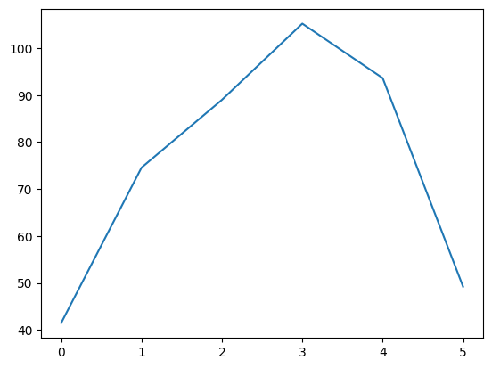
df.Diff.plot()
<Axes: >
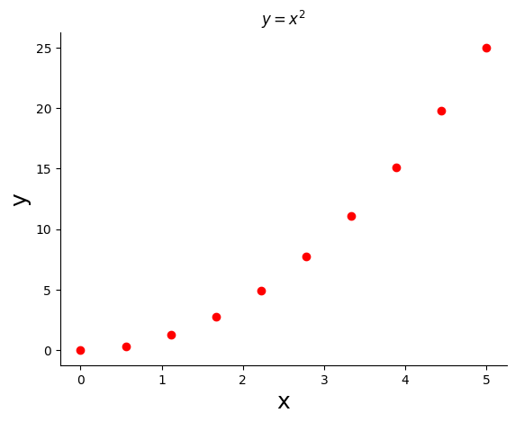
x = np.linspace(0, 5, 10)
y = x**2
x
array([0.        , 0.55555556, 1.11111111, 1.66666667, 2.22222222,
       2.77777778, 3.33333333, 3.88888889, 4.44444444, 5.        ])
plt.figure()
plt.plot(x, y, "ro")
plt.xlabel("x", fontsize=18)
plt.ylabel("y", fontsize=18)
plt.title("$y = x^2$")

sns.despine()
Great documentation and basic tutorial available from the lectures of Robert Johansson
1.4.1. Seaborn#
Seaborn is a Python visualization library based on matplotlib. It provides a high-level interface for drawing attractive statistical graphics.
import seaborn as sns
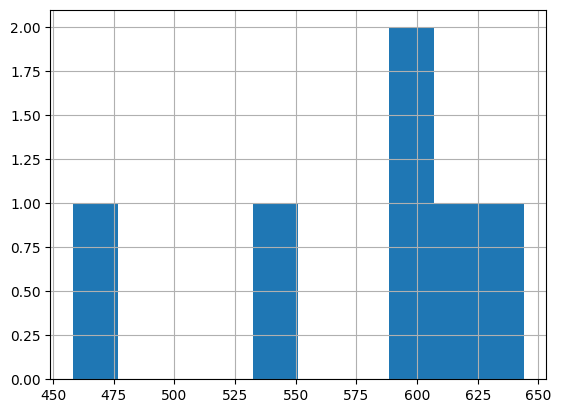
df.High.hist()
<Axes: >
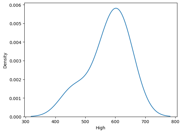
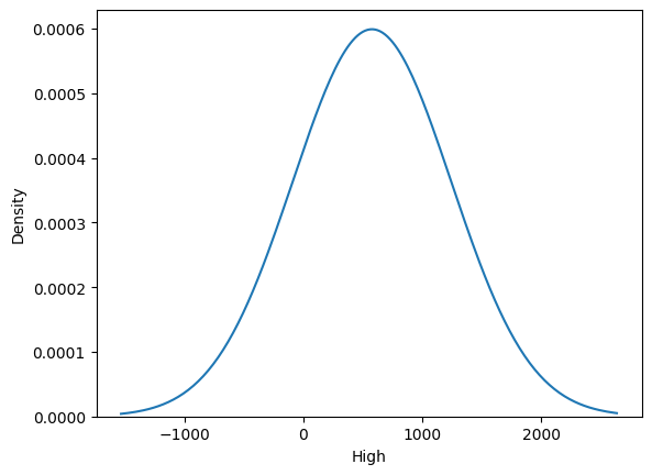
sns.kdeplot(df.High)
<Axes: xlabel='High', ylabel='Density'>
sns.kdeplot(df.High, bw=10)
/var/folders/wm/5gv37br900l73y63tjf8sr1r0000gn/T/ipykernel_13285/1765152266.py:1: UserWarning:

The `bw` parameter is deprecated in favor of `bw_method` and `bw_adjust`.
Setting `bw_method=10`, but please see the docs for the new parameters
and update your code. This will become an error in seaborn v0.13.0.

  sns.kdeplot(df.High, bw=10)
<Axes: xlabel='High', ylabel='Density'>
for loop

